Optimization Up

Media planners usually use Excel and formulas to create detailed media plans, capturing how much investment is put behind each media channel, each market, each month ..etc. Then perform analysis using static benchmarks to see the impact on leads, sales, and return on investment. This process is tricky as it requires a lot of time and experience to get it right, especially when leveraging historical data in making predictions.

Today, I will show you how to use your existing dataset in BigQuery to estimate any time-series value using the ARIMA ML model. This should enable you to streamline and automate your client’s media planning & forecasting. We will look at 2 use cases:

1- Forecasting the number of transactions on a daily basis (Single Time Series)

2- Forecasting the CPC per advertising channel on a daily basis (Multiple Time Series)

BigQuery supports creating and executing machine learning models using just SQL. You can use BiqQuery ML to train models on data already in BiqQuery without any deep knowledge of machine learning. The tool supports many machine learning models that can be deployed on any kind of dataset. The model that we will be utilizing today is Time Series (ARIMA).

Forecast Single Time Series (Transactions)

In this use case, we will try to forecast the number of transactions for an e-commerce store on a daily basis. The steps to create the model are as follows:

1- Prepare the data

The first step in creating the ML model is to check and clean your dataset. Keep in mind, the more data the better predictions the model can make. In this exercise, I will be taking 1 year of data, The raw dataset looks like this:

SELECT
  date,
  SUM(transactions) AS transactions
FROM
  `myproject.mydataset.mytable`

GROUP BY
  date
ORDER BY
  date DESC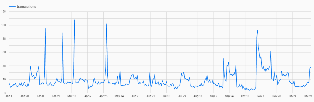

From the chart, you can see there are some spike patterns throughout the year, usually driven by the holiday season and tactical campaigns.

2- Train the Model

Now it’s time to create and train the model. Training the time-series model is straightforward. 

CREATE OR REPLACE MODEL
  `myproject.mydataset.myfirstmodel` OPTIONS(model_type= 'ARIMA',
    time_series_data_col='transactions',
    time_series_timestamp_col='date',
    data_frequency='DAILY' ) AS
SELECT
  CAST(FORMAT_DATE("%Y-%m-%d", DATE(date)) AS TIMESTAMP) AS date,
  SUM(transactions) AS transactions,
FROM
  `myproject.mydataset.mytable`
GROUP BY
  1
ORDER BY
  1,
  2 DESC

model_type: Specifies the model type. To create a time series model, set model_type to 'ARIMA'.

time_series_data_col: The data column name for time series models we want to forecast, in this case, we want to forecast ‘transactions’

time_series_timestamp_col: The timestamp column name for time series models, in this case, we had to convert the date to timestamp as it’s a string

data_frequency: The data frequency of the input time series, could be: ‘PER_MINUTE’ | ‘HOURLY’ | ‘DAILY’ | ‘WEEKLY’ | ‘MONTHLY’ | ‘QUARTERLY’ | ‘YEARLY’

3- Evaluating the model

After creating the model, you can use the ML.EVALUATE function to see the evaluation metrics of all the created models

SELECT
  * 
FROM
  ML.EVALUATE(MODEL bqmlforecast.arima_model)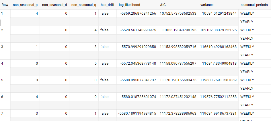

See the documentation here for the definition of each metric.

4- Make predictions using the model

To make predictions, we use ML.FORECAST, which forecasts the next n values, as set in the horizon. You can also change the confidence_level, the percentage that the forecasted values fall within the prediction interval. The model below forecasts 90 days into the future with a prediction interval of 80%

SELECT
  *
FROM
  ML.FORECAST(MODEL `myproject.mydataset.myfirstmodel`,
    STRUCT(90 AS horizon,
      0.8 AS confidence_level))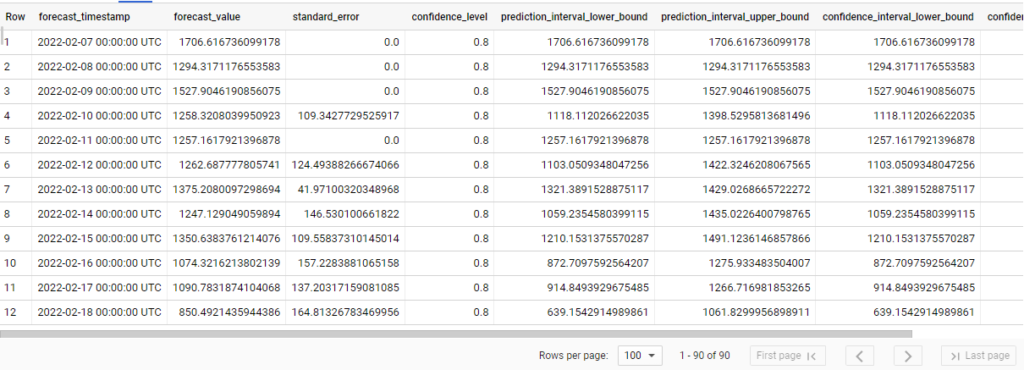

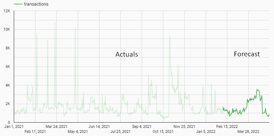
And now we have the transactions forecast for the next 90 days. Each forecasted value also shows the upper and lower bound of the prediction_interval, given the confidence_level. If we plot the forecasted predictions next to the actuals, this is how it looks like:

Forecast Multiple Time Series (CPC per Channel)

You can train a time series model to forecast a single series, or forecast multiple fields at the same time. To forecast multiple time series, all we have to do is include a new option called time_series_id_col and add the dimension we want. In this example, I will be adding ‘channel’ which refers to the advertising channel to forecast the cost per click (CPC).

CREATE OR REPLACE MODEL
  `myproject.mydataset.mysecondmodel` OPTIONS(model_type= 'ARIMA',
    time_series_data_col='cpc',
    time_series_timestamp_col='date',
    time_series_id_col='channel',
    data_frequency='DAILY' ) AS
SELECT
  CAST(FORMAT_DATE("%Y-%m-%d", DATE(date)) AS TIMESTAMP) AS date,
  data_source AS channel,
  SUM(spend) / SUM(clicks) AS cpc,
FROM
  `myproject.mydataset.mytable`
GROUP BY
  1,
  2
ORDER BY
  date,
  cpc DESC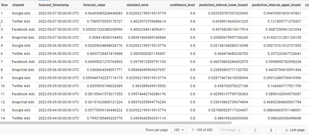

Viola! we now have the CPC forecast for each channel in the next 90 days. To create fresh time-series forecasts based on the most recent data, you can use scheduled queries to automatically re-run your SQL queries, which includes your CREATE MODEL, ML.EVALUATE or ML.FORECAST queries