

5 Advanced Excel Formulas for PPC Professionals
Excel is one of the most powerful tools that can make you better and faster in PPC management, it’s a very crucial skill for every digital marketer. In this post, we’ll go over 5 formulas that will make your life much easier, starting from building campaigns, writing ads, and analyzing data sets.
1. IF contains this then that
The formula checks if a cell contains specific text and returns a value you determine for TRUE and another value for FALSE.
Syntax
=IF(ISNUMBER(SEARCH(substring, cell)), text, text)
The SEARCH function returns the position of the search string when found. And ISNUMBER returns TRUE for numbers and FALSE for anything else. Wrapping both formulas in IF can allow you to return specific values instead of TRUE and FALSE.
Example
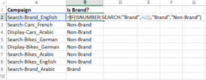
Let’s say, you want to analyze the performance of your brand campaigns vs non-brand campaigns. And you do include in your campaigns naming a unique identifier for brand-related terms which is the word “brand”. You want to check if the campaign contains brand then returns “Brand” and if not then return “Non-Brand”.
=IF(ISNUMBER(SEARCH("Brand",A2)),"Brand","Non-Brand")
2. Extract text before/after a specific character
To split a text string at a specific character, we can use a combination of LEFT, RIGHT, and FIND functions.
Syntax
=LEFT(A2,FIND("_",A2)-1)
This splits the text before the underscore character. The FIND function is to locate the underscore(_) in the text, then we subtract 1 to move back to the “character before the special character.
=RIGHT(A2,LEN(A2)-FIND("_",A2))
This splits the text after the underscore character. The FIND function is to locate the underscore(_) in the text, then we subtract the length of the cell (using LEN) from the index location of the underscore character, the result gives us the number of characters to return from the right.
Example
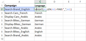
You want to pull out the language out of the campaign names which is located after a specific character “_”. You can use the formula below:
=RIGHT(A2,LEN(A2)-FIND("_",A2))
3. SUMIF/SUMIFS
SUMIF adds all numbers in a range of cells based on one criteria, while SUMIFs sum cells that meet multiple criteria.
Syntax
=SUMIF( range, criteria, [sum_range] )
=SUMIFS (sum_range, range1, criteria1, [range2], [criteria2], ...)
- sum_range : The range to be summed.
- range : The range of cells that you want to apply the criteria against.
- criteria : The criteria used to determine which cells to add.
Example
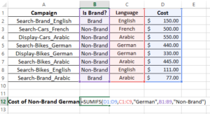
From our last example, let’s you want to know the amount spent on German non-brand campaigns. Your formula can look like below:
=SUMIFS(D1:D9,C1:C9,"German",B1:B9,"Non-Brand")
4. Substitute & Concatenate
The SUBSTITUTE function replaces text in a given string, while CONCATENATE joins multiple texts together.
Syntax
=SUBSTITUTE (cell, old_text, new_text)
=CONCATENATE(text,text,text)
Example
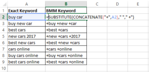
You want to create broad match modifier keywords by appending the plus to your exact match type keywords. By combining SUBSTITUTE and CONCATENATE, you can append the + to the beginning of the text and replace the space by ” +”.
=SUBSTITUTE(CONCATENATE("+",A2)," "," +")
5. Index & Match
They look for specific information in your worksheet, they are similar to the popular VLOOKUP function. However, INDEX and MATCH are more useful since they are dynamic, they respond to change. This means deleting or adding columns in your search range won’t screw your formulas, unlike the VLOOKUP function which doesn’t respond to change.
Syntax
=INDEX(range, MATCH(lookup_value, lookup_range, match_type))
- range: This is where you’d like to look up a given value.
- lookup_value: This is what you want to look up for.
- lookup_range: This is the range of your given value.
- match_type: Most of the times, it will be exact 0.
Example
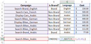
Let’s say you want to find the cost of a specific campaign in your data set, your formula can look like below:
=INDEX(D1:D9,MATCH(A11,A1:A9,))

Entrepreneur focused on building MarTech products that bridge the gap between marketing and technology. Check out my latest product GA4 Auditor and discover all my products here.
You can use advanced or complicated formulas built in Dose for Excel without even writing it, the tool will write it for you:
https://www.zbrainsoft.com/Formula-Helper.html
how to change cell value ( many cells ) to comments at once??
http://www.ju.edu.jo